
AI summary
The article discusses the critical role of storage architecture in determining system performance, cost, and reliability. It contrasts local and distributed storage systems, highlighting that local storage offers speed but lacks redundancy, while distributed storage provides durability at the cost of increased latency. The piece explains various drive types, including HDDs and SSDs, and their respective performance characteristics. It also outlines redundancy models, emphasizing the differences between local redundancy, typically managed by RAID, and distributed redundancy, which relies on data distribution across multiple nodes. The article concludes by categorizing data into hot and cold storage, recommending that organizations align their storage solutions with data access patterns and failure management strategies.
Your storage setup decides how your system behaves when people actually use it. It decides whether a service keeps up under load, how much you end up paying for capacity, and how much trouble you’re in when something breaks. Though some might think of storage as just a box you stick data into – one shape, one behavior, one line on a diagram – it’s really nothing like that.
Under the surface, storage is defined by two things: where the data physically lives and what has to happen every time you touch it. Those two choices govern everything else – latency, failure modes, durability, and cost per terabyte. They’re also the reason one architecture survives node failures without blinking, while another falls over after a single busy hour.
Local vs Distributed Storage
Every storage system starts with the same question: does the data stay on the machine that uses it, or does it live across several machines? That dictates most of the performance profile and almost all of the failure behavior.
Local Storage
Local storage is the simplest. It’s a drive plugged into the same server that runs the workload. The data never leaves the box. Reads and writes go straight through the controller and hit the device with no network in between. That’s why it’s also the fastest option you can get. The path is short, the latency is minimal, and nothing waits on another node to confirm anything.
The downside is that if the server dies, the data becomes unavailable. Data replication could be provided at the RAID level within the server.
Distributed Storage
Distributed storage flips the priorities. Instead of trusting one machine, the system spreads data across multiple servers and keeps track of every piece. There’s a special software layer that decides where each chunk goes, how many replicas exist, and what happens when a disk or an entire node disappears. To the application, it all looks like one logical volume. But, under the hood, it’s thousands of moving parts.
The trade-off is latency. Every write has to travel across the network and wait for replication. Reads may hit a different node each time. The cluster needs time to coordinate, rebalance, and repair.
But this is also what makes them dependable. If a node collapses, the system keeps serving data and quietly rebuilds the missing pieces in the background.
Where They Meet
Once you compare local and distributed storage side by side, the pattern becomes obvious. Every design lives somewhere between two promises: IO speed and data availability. You can optimize for one, or you can optimize for the other, but modern infrastructures use both. Active working sets, databases, I/O-heavy workloads – prefer fast local drives or high-performance block volumes. Durable data – backups, archives, long-tail media, logs – typically lives on HDD-based distributed storage that can survive hardware failure.
Learn how we build custom infrastructure that matches the real behavior of your data
Drive Types and Technologies
Once you know where data lives, the next variable is what you store it on. Drives come in a large variety. They behave differently under load, and those differences shape which workloads feel fast and which ones fall apart.
HDD – Mechanical, Cheap, Predictable
HDDs store data on spinning magnetic platters. A small arm with a read/write head moves to the right sector each time you request data.

That physical movement is the bottleneck:
- Sequential access (big files in order) is fine because the head barely moves.
- Random access (small files everywhere) is slow because the head has to reposition for every operation.
Driven by mechanics, HDDs deliver:
- Low IOPS (I/O operations per second) – usually ~100–150.
- High capacity – 20–26 TB per disk.
- Lowest cost per TB.
They’re perfect for workloads where latency doesn’t matter much: archives, backups, long-tail content.
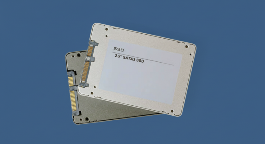
SSD – Flash Without the Mechanical Penalty
SSDs use NAND flash, which is just electronic memory arranged in blocks.
No movement, no arm, no platter. Access is effectively instantaneous.
- Random reads and writes are fast.
- Latency drops from milliseconds to microseconds.
- IOPS jump to tens of thousands.
But a lot of the speed and functionality also depends on the interface on the hardrive. So, let’s explain them properly.
SATA – Serial ATA
SATA is the simplest, oldest, and slowest interface used in servers.
It was designed in the mechanical era and has these limits:
- One command queue → only one operation in flight at a time.
- ~550 MB/s max throughput (serial bottleneck).
- Affordable, widely supported, reliable, but not built for high concurrency.
So, when an SSD has SATA it is fine for moderate workloads, but cap the performance of flash because the interface itself is slow.
SAS – Serial Attached SCSI
SAS is the enterprise version of SATA. It’s still serial, but with key differences:
- Multiple parallel command queues → many operations at once.
- ~1400 MB/s max throughput
- Full-duplex → read and write simultaneously.
- Higher rotational speeds for HDD (10k–15k RPM) and better latency.
- Dual-port capability → redundancy paths in server backplanes.
SAS handles more concurrency and more predictable throughput than SATA, so it’s used where reliability and steady performance matter – even if the underlying media is still HDD or basic SSD.
NVMe – Flash at Full Speed (via PCIe)
NVMe is not an interface like SATA/SAS. It’s a protocol designed specifically for flash, running on PCIe lanes — the same high-bandwidth bus used by GPUs and fast NICs.

PCIe gives NVMe:
- Parallelism: thousands of independent queues
- Massive bandwidth: multi-GB/s
- Low latency: direct connection to CPU
NVMe finally lets flash perform at its real speed, instead of being throttled behind legacy serial interfaces. This is why NVMe is the hardware foundation of hot storage – any workload that’s deeply sensitive to latency.
There are other, of course, storage media beyond HDD, SSD, and NVMe, such as optical disks, tape libraries, and niche archival formats. Tape in particular is still widely used for large-scale cold storage because it offers extremely low cost per terabyte and long retention times. But for this article, we focus on the devices that actually sit and power behind enterprise storage architectures.
Access Patterns

Sequential Access
Sequential access is the easy path – large, continuous reads or writes. HDDs handle this well because the head barely moves. The hardware is slow, but the pattern is friendly. This is the so-called cold storage’s natural territory: big files, predictable reads, low urgency.
Random Access
Random access is the stress test – small blocks scattered across the disk. Web apps serving images, databases updating rows, CDNs delivering thousands of objects per second. HDDs choke here because the head is constantly repositioning. Flash doesn’t have that problem. SSDs and NVMe drives jump between memory cells instantly. That’s why they deliver tens or hundreds of thousands of IOPS while HDDs stall at a few hundred.
Mixed Loads
Most real workloads are 70/30 or 80/20 read/write mixes with mostly random patterns. This is exactly where SSD and NVMe outperform mechanical drives by orders of magnitude.
We can design a custom stack that stays fast under load instead of collapsing under concurrency
Redundancy Models: Local vs Distributed
The next question is how it survives hardware failure. And the gap between local and distributed solutions is bigger than most diagrams suggest. They aren’t variations of the same idea – they operate on completely different assumptions about what can break and how often it will.
Local Redundancy
On a single server, storage redundancy is usually supplied by RAID. It’s the oldest approach we have for keeping a system alive when a disk fails, and it comes in a handful of forms that all follow the same principle: several physical drives pretend to be one or more redundant logical drives.
Mirroring is the simplest version. Two drives store the same data sector-for-sector. If one dies, the other takes over without the system even noticing. It’s clean and predictable, but more expensive in terms of usable space. You’re throwing away half your capacity for the privilege of not rebooting during a drive swap.
Parity arrays came next. Instead of duplicating everything, the system spreads data across a set of drives and calculates extra parity blocks that can be used to reconstruct whatever goes missing. RAID 5 relies on a single parity block per stripe, which works fine until disks become large enough that rebuild time becomes a problem. Modern HDDs need time to rebuild, and during that window, the entire array is one failure away from collapsing. RAID 6 tries to address this by adding a second parity block so you can survive two failures, but the underlying problem remains: you’re asking a handful of drives in a single chassis to carry all the risk.
Striped mirrors – RAID 10 – are what people use when they want speed, predictability, and simple failure behavior. They combine striping for performance and mirroring for safety, and they work well on solid-state storage. But they still share the same fundamental limitation: the data is tied to the server. If the controller locks up, if the power supply takes two disks with it, if the entire machine disappears behind a networking failure, RAID offers no protection. It is a tool for uptime, not durability.

Local redundancy keeps a machine running, not data alive.
Distributed Redundancy
Distributed systems take a different approach. Instead of assuming one machine and trying to protect it from drive failures, they assume that machines will fail constantly and design the storage layer so the system continues operating anyway.
When a write enters a distributed cluster, it doesn’t land on a single disk. It’s broken into pieces and placed across multiple servers according to a durability rule. If a node dies, the cluster keeps serving data from the remaining pieces. Rebuilds happen in the background.
The simplest model is replication: keep multiple full copies on independent nodes. Three copies are the common baseline. It’s more demanding in terms of capacity, but it’s fast and predictable. Most hot data in distributed systems lives on replicated volumes; for that reason – you pay the overhead because latency matters.
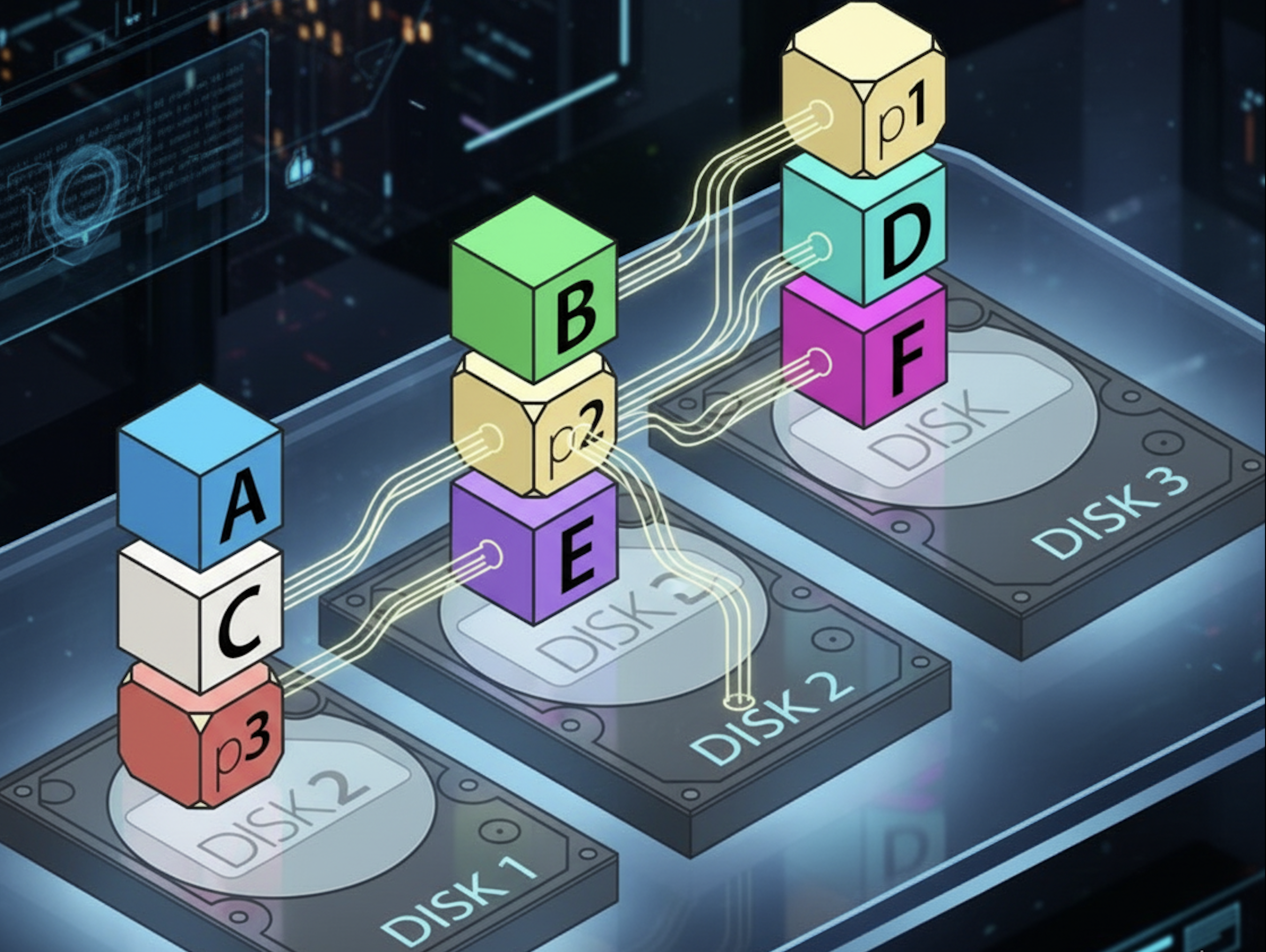
But replication becomes expensive when you’re storing petabytes. That’s why distributed systems use erasure coding for colder tiers. It looks a lot like RAID 6 at first glance – data and parity fragments spread across several drives – but the scale and behavior are completely different. Instead of placing those fragments on disks inside one box, they’re placed across servers, racks, and other failure domains. Instead of a single controller doing all the work, the cluster coordinates recovery. Instead of one parity block per stripe, you can choose whatever ratio you want: 4+2, 8+3, 10+4. Lose any two, or three, or four fragments, depending on the scheme, and the system rebuilds the missing data mathematically.
Erasure coding cuts overhead dramatically. A 4+2 layout survives two simultaneous failures with only a 1.5× penalty instead of replication’s 3×. That’s why it’s used for massive object stores, archival systems, and distributed clusters where durability matters more than immediate access speed.
Distributed redundancy doesn’t protect a machine; it protects the data itself. It shifts durability from hardware to math, from controllers to cluster logic, and from the scale of a single box to the scale of an entire environment. That’s why systems like Ceph are resilient. They assume the disks will collapse – constantly – and build around the idea.
Distributed Storage in Practice
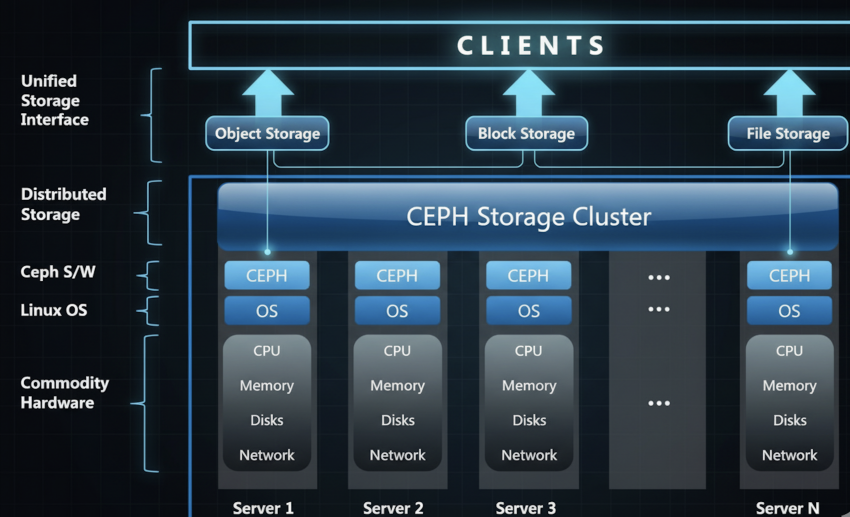
Once you leave the world of single servers, storage stops being a device and becomes a service. A distributed system is just a set of ordinary machines tied together by software that decides where every byte goes and how many copies exist.
A system like Ceph is a good example. Every node has its own disks – HDD for capacity, SSD or NVMe for speed – and Ceph glues them into several logical pools. The application never sees individual disks. It sees a virtual volume or a bucket. Writes come in, get split into pieces, and those pieces are placed on different nodes according to replication or erasure-coding rules. If a node dies, the cluster doesn’t pause. It serves data from the remaining copies and quietly rebuilds the missing pieces in the background.
This is where availability and durability come into play. Availability is whether you can read or write right now. Durability is whether the data survives hardware failure. Distributed systems are designed to trade a bit of latency for extreme durability – because a few extra milliseconds is tolerable, but losing data isn’t.
They also offer multiple access models depending on the needs of the workload. This category defines how data is structured and presented to the application or user. It is typically an architectural choice made within NAS, SAN, and cloud environments.
| Access Method | Structure | Used For | Key Features |
| File Storage | Data is organized into a hierarchical structure (files inside folders/directories). | Documents, file shares, media libraries (common in NAS and local drives). | User-friendly, easy sharing, limited scalability compared to Object. |
| Block Storage | Data is broken into evenly sized blocks, each with a unique address, independent of the operating system. | Databases, Virtual Machines (VMs), transaction processing (common in SAN). | Fastest performance, low latency, raw storage blocks controlled by the server OS. |
| Object Storage | Data is stored as a self-contained unit (object) bundled with metadata (user-defined tags) and a unique identifier. Flat structure (no folders). | Unstructured data, media archives, web content, Big Data (common in Cloud Storage like Amazon S3). | Massive scalability, highly distributed, accessed via HTTP APIs. |
Underneath, it’s all the same cluster. The interface is just the mask that the application sees.
Distributed storage makes data safer by spreading risk across machines, racks, and other failure domains, and by treating rebuilds as routine background work instead of emergencies.
Hot and Cold Storage: What the Terms Actually Mean
By the time you understand drive behavior, access patterns, and how distributed systems keep data alive, the idea of “hot” and “cold” storage becomes obvious. These categories are a natural result of how data behaves and what the system has to guarantee when someone accesses it.
Hot storage is designed for data that is accessed frequently and requires an immediate response. It represents the highest-performing – and typically the most expensive – storage tier.
| Characteristic | Description |
| Access Frequency | High (daily, hourly, or constantly). |
| Performance | High speed, low latency (measured in milliseconds or less). |
| Cost | Highest cost per GB. |
| Primary Technology | SSDs (Solid State Drives) in SANs or high-performance flash arrays, high-speed cloud storage tiers. |
| Use Cases | Transactional databases (e.g., customer orders), active virtual machines (VMs), operating systems, mission-critical applications, real-time analytics. |
Cold storage is designed for data that is accessed rarely, if ever, and can tolerate high latency during retrieval. It is the lowest-cost storage tier and is used primarily for long-term retention, compliance, and archival datasets.
| Characteristic | Description |
|---|---|
| Access Frequency | Low (monthly, quarterly, or not at all). Retrieval may take some time. |
| Performance | Low throughput, high latency. |
| Cost | Lowest cost per GB. |
| Primary Technology | Magnetic tape libraries, high-density HDD systems, and deep archival cloud tiers (e.g., AWS Glacier Deep Archive). |
| Use Cases | Regulatory archives (financial records, medical records requiring 7+ years), long-term media backups, genomic datasets, research data requiring preservation |
We can sum this up like this:
- Hot data is random, concurrent, and latency-sensitive.
- Cold data is sequential, infrequent, and patient.
A video catalog is cold. The segments being streamed right now are hot. Long-tail CDN images are cold. The 1% that get fetched constantly are hot. Backup copies of the video catalog and CDN images are cold.
Note on JBOD
In the context of everything we’ve discussed, it’s also worth mentioning JBOD – “Just a Bunch of Disks.”
It’s exactly what it sounds like: a server or enclosure filled with individual drives that the system exposes one by one, with each disk remaining completely independent. In other words, it’s raw storage presented as separate devices.
JBOD is the simplest way to expand storage alongside server. It doesn’t add redundancy or improve performance; it simply gives the machine more physical drives to work with. JBOD is useful when you need capacity in a chassis and the redundancy is handled somewhere else – by the application, the filesystem, or a distributed storage layer. In that sense, JBOD isn’t a storage model at all. It’s the physical baseline on top of which everything else – RAID, replication, erasure coding – actually happens.
Conclusion.
If you understand where your data lives, how often it’s accessed, and what failure looks like in your environment, the right storage architecture becomes obvious.
Put the fast stuff where latency hurts. Put the durable information where the cost matters more. And let the system do the rest.
If you want help mapping your workloads to the right storage tiers – or you’re building something that needs to scale without falling apart – reach out. Being experts in building all aspects of custom infrastructure, we can design a storage layout that matches the real behavior of your data.


